Week 1. Hyperparameter tuning, Regularization and Optimization

1. Data

Divide all the data into three parts:

• the training set: to train the NN
• the develop (dev) set: to tune the model
• the test set: to test the model’s performance (don’t tune the model according to its results, that’s what dev set is for)

Empirical division strategy:

Small data: 0.6, 0.2, 0.2

Big data: 0.98, 0.01, 0.01 (e.g.)

⚠️ The data sets should have the same distribution. E.g. an classifier may be trained by high-resolution images but the dev & test data sets are

2. Bias & Variance

Bias & Variance

Bias: the difference between the estimator’s expected value and the true value of hte parameter being estimated (Ref). High bias $\rightarrow$ under fitting

Variance: an error from sensitivity to small fluctuations in the training set (Ref). High variance $\rightarrow$ over fitting

High bias and high variance can coexist, especially for multi–dimension data.

Bias–Variance Tradeoff

• Cross–Validation
• or mean squared error (MSE)

Optimal Error / Bayes Error

Def: the error of an ideal model, or the lowest possible prediction error that can be achieved (Ref)

Used as a reference for evaluating the performance of a model.

3. How to Deal with Bias and Variance

If high bias (from training set performance):

• Bigger NN
• Longer training
• Other NN architecture

If high variance (from dev set performance):

• More data
• Regularization
• Other NN architecture

4. Regularization

To address the problem of overfitting

Regularization works well when there are lots of slightly useful features.

The Formula

Hyper parameter $\lambda$, the regularization parameter.

The updated cost function:

$\large J(w,b) = \frac{1}{m} \sum\limits_{i=1}^{m} L(\hat{y}^{(i)}, y^{(i)}) + \frac{\lambda}{2m} \sum\limits_{l=1}^L \parallel w^{[l]} \parallel^2_2$

in which $\large \parallel w^{[l]} \parallel^2_2 = \sum\limits_{i=1}^{n^l}\sum\limits_{j=1}^{n^{[l-1]}} (w_{i,j}^{[l]})^2$ is the L2 regularization, and the value is the squared Euclidean norm; the matrix norm is called the “Frobenius norm”. And thus $\large J_{regularized} = \small \underbrace{-\frac{1}{m} \sum\limits_{i = 1}^{m} \large{(}\small y^{(i)}\log\left(a^{[L](i)}\right) + (1-y^{(i)})\log\left(1- a^{[L](i)}\right) \large{)} }_\text{cross-entropy cost} + \underbrace{\frac{1}{m} \frac{\lambda}{2} \sum\limits_l\sum\limits_k\sum\limits_j W_{k,j}^{[l]2} }_\text{L2 regularization cost}$

Also, the updated derivatives:

$\large \mathrm{d}w^{[l]} = \frac{1}{m} \mathrm{d} z^{[l]} a^{[l-1]T} + \frac{\lambda}{m}w^{[l]}$

$\large w^{[l]} := (1-\frac{\alpha \lambda}{m}) w^{[l]} - \frac{\alpha}{m} \mathrm{d} z^{[l]} a^{[l-1]T}$

Why It Works

L2-regularization relies on the assumption that a model with small weights is simpler than a model with large weights. Thus, by penalizing the square values of the weights in the cost function you drive all the weights to smaller values. It becomes too costly for the cost to have large weights! This leads to a smoother model in which the output changes more slowly as the input changes.

5. Dropout

To address the problem of overfitting

Always used in CV

Dropout is only used for the test set.

Basic idea:

Randomly eliminate neurons in the hidden layers at each iteration.

Implementation

Common method: inverted dropout

• Set the hyper parameter “keep probability”, it may be difference for different layers
• Generate a random matrix with the same shape of the layer
• set 1 to items higher than the keep-prob, 0 to the others (generate a “mask”)
• multiply the random matrix with the original neuron matrix A
• Set A = A/keep-prob to keep the same expectation

Backward propagation:

• Shut down the same neurons by applying the same mask to the derivative matrix.
• Divide the derivative matrix by the keep–probability

Why It Works

Equivalent to fitting with a smaller NN.

The model will spread the weights on the neurons in case some of them are eliminated

6. Other Regularization Methods

To address the problem of overfitting

1. Enlarge the data.

   e.g. for images, flip/random distortion the images to create “fake examples”

2. Early stopping

   Stop training at the iteration with best performance (lowest J)

   Drawbacks: optimizing J and doing regularization at the same time, not up to the orthogonalization method (think about one task at a time), thus cannot solve the problems separately.

7. Optimization

1. Normalize the Training Set

$\large x := \frac{x-\mu}{\sigma}$

where $\large \mu = \frac{1}{m} \sum \limits_{i=1}^{m}x^{(i)}$, $\large \sigma^2 = \frac{1}{m} \sum \limits_{i=1}^{m}x^{(i)2}$

2. Vanishing/Exploding Gradients

Def: the derivatives become extremely large or small when training a deep NN

Solution:

• the larger input features $n$, the smaller $w_i$;

• initialize $w_i$ with $\mathrm{Variance}(w_i) = \frac{1}{n}$, or $\frac{2}{n}$ for ReLU

Implementation notes:

1
w[l] = np.random.randn(shape_of_w[l]) * np.sqrt(1/n[l-1]) # 2/n[l-1] for ReLU

3. Gradient Checking

To check whether the back–propagation implementation is right by checking verifies closeness between the gradients from backpropagation and the numerical approximation of the gradient (computed using forward propagation).

1. Reshape each $W$, $b$ in to vector $\Theta$; $\mathrm{d}W$, $\mathrm{d}b$ into vector $\mathrm{d}\Theta$
2. Thus $\large J(W^{[1]}, b^{[1]}, \dots, W^{[i]}, b^{[i]}, \dots, W^{[L]}, b^{[L]}) = J(\Theta) = J(\Theta_1, \dots, \Theta_i, \dots)$
3. for each $i$, let $\large \mathrm{d}\Theta_{approx}^{[i]} = \frac{J(\Theta_1, \dots, \Theta_i + \epsilon, \dots) - J(\Theta_1, \dots, \Theta_i, \dots)}{2\epsilon}$, which is the approximation of $\large \frac{\partial J}{\partial \Theta_i}$
4. Check if $\large \frac{\parallel\mathrm{d}\Theta_{approx} - \mathrm{d}\Theta \parallel_2}{\parallel\mathrm{d}\Theta_{approx} \parallel_2 + \parallel\mathrm{d}\Theta \parallel_2} < \epsilon = 10^{-7}$
   • $\sim 10^{-7}$: great
   • $\sim 10^{-5}$: some components may be too large/have bugs
   • $\sim 10^{-3}$: careful of BUGs!!!

Implementation Notes:

1. Only use to debug, NOT while training (computational resources consuming).
2. If failed, look at components to identify bug.
3. Remember regularization if used during training.
4. Doesn’t work with dropout.
5. Run at random initialization; perhaps again after some training.

Week 2. Optimization Algorithms

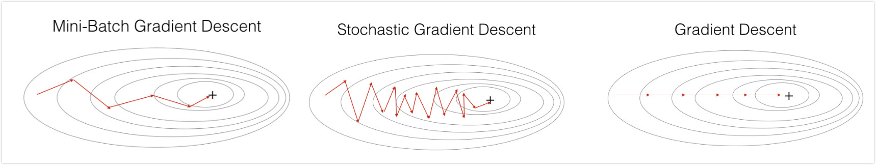
1. Mini–batch Gradient Descent

To speed up the training

Divide the training set into smaller “batches”, and update the parameters after one mini-batch is trained.

• batch size = size of training set $\rightarrow$ batch gradient
  • good for small training set (< 2000)
  • smooth curves of J vs. #iterations plot
  • slow for large training set
  • Sample:

    1
    2
    3
    4
    5
    6
    7
    8
    9
    10
    11
    12
    13
    X = data_input
    Y = labels
    parameters = initialize_parameters(layers_dims)
    for i in range(0, num_iterations):
      # Forward propagation
      a, caches = forward_propagation(X, parameters)
      # Compute cost.
      cost += compute_cost(a, Y)
      # Backward propagation.
      grads = backward_propagation(a, caches, parameters)
      # Update parameters.
      parameters = update_parameters(parameters, grads)
              
    

• batch size = 1 $\rightarrow$ Stochastic batch (just train one example then update the parameters, and move to the next example)

  • loose speedup from vactorization

  • the curve is extremely noisy

  • Sample:

    1
    2
    3
    4
    5
    6
    7
    8
    9
    10
    11
    12
    13
    X = data_input
    Y = labels
    parameters = initialize_parameters(layers_dims)
    for i in range(0, num_iterations):
        for j in range(0, m):
            # Forward propagation
            a, caches = forward_propagation(X[:,j], parameters)
            # Compute cost
            cost += compute_cost(a, Y[:,j])
            # Backward propagation
            grads = backward_propagation(a, caches, parameters)
            # Update parameters.
            parameters = update_parameters(parameters, grads)
    

• mini batch usually have size between the above and is the power of 2 (64 ~512)
  • good for large training set
  • the curve is noisier than batch gradient descent, but smoother than Stochastic batch
  • take advantage of the speedup from vectorization
  • make progress without processing the entire training set

2. Gradient Descent with Momentum

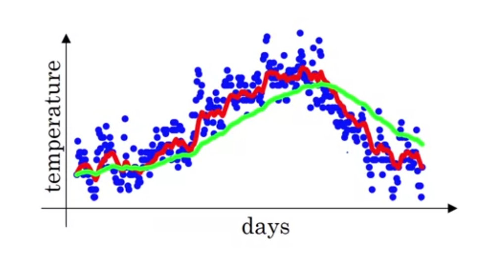
1. Exponentially Weighted Averages

Definition

$\theta_t$ is the value, and $v_t$ is the corresponding EWA, then:

• $\large v_0 = 0$

• $\large v_t = \beta v_{t-1} + (1-\beta) \theta_t$, $(\beta < 1)$

$v_i$ is approximately the average of the $\large \frac{1}{1-\beta}$ data points;

the curve becomes smoother and shifts to right ( latency) when $\beta$ increases.

Intuition

$\large (1-\epsilon)^{\frac{1}{\epsilon}} = \frac{1}{e} \approx 0.37$

Thus it takes about 1/$\epsilon$ items before the weight decay below $e^{-1}$.

Bias Correction

For the initial phase, update the original $v_t$ with $\large \frac{v_t}{1-\beta^t}$.

Unnecessary for larger t.

Not really matters whether to correct this.

2. Gradient Descent with Momentum

Always works faster than the standard gradient descent algorithm

Why it works:

Smooth out the steps of gradient descents perpendicular to the direction towards minimum, but save the progress towards the minimum.

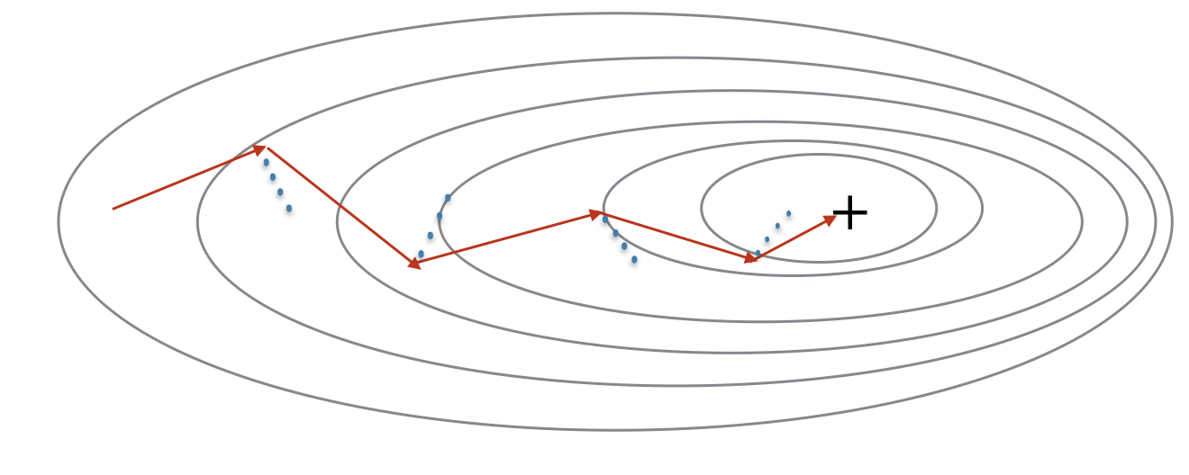
Use EWA to update the gradient. Hyperparameter, $\beta$

Implementation:

• Initialize $v_{\mathrm{d} w} = 0$, and $v_{\mathrm{d} b} = 0$

• On iteration of t:

  • compute $\mathrm{d}w$, $\mathrm{d}b$ on current mini–batch

  • compute $\large v_{\mathrm{d} w} = \beta v_{\mathrm{d}w} + (1-\beta) \mathrm{d}w$; $\large v_{\mathrm{d} b} = \beta v_{\mathrm{d}b} + (1-\beta) \mathrm{d}b$

  • update $w$ with $\large w := w - \alpha v_{\mathrm{d} w}$ and $\large b := b - \alpha v_{\mathrm{d} b}$

Often choose $\beta = 0.9$

3. Root–Mean–Square Prop (RMSprop)

Implementation:

• On iteration of t:
  • compute $\mathrm{d}w$, $\mathrm{d}b$ on current mini–batch
  • compute $\large S_{\mathrm{d} w} = \beta S_{\mathrm{d}w} + (1-\beta) \mathrm{d}w^2$; $\large S_{\mathrm{d} b} = \beta S_{\mathrm{d}b} + (1-\beta) \mathrm{d}b^2$ (element wise squaring)
  • update $w$ with $\large w := w - \alpha \frac{\mathrm{d} w}{\sqrt{S_{\mathrm{d} w}}}$ and $\large b := b - \alpha \frac{\mathrm{d} b}{\sqrt{S_{\mathrm{d} b}}}$

⚠️ To avoid divided by zero, always use $\large \sqrt{S_{\mathrm{d} b}} + \epsilon$ ($\large \epsilon = 10^{-8}$) instead of just $\large \sqrt{S_{\mathrm{d} b}}$

Why it works:

Similar to the gradient descent with momentum.

4. Adaptive Moment Estimation (Adam) Optimization Algorithm

A combination of momentum and RMSprop

Very efficient!

Implementation:

• Initialize $v_{\mathrm{d} w} $, $v_{\mathrm{d} b}$, $S_{\mathrm{d} w} $, and $S_{\mathrm{d} b}$ to zero
• On iteration of t:
  • compute $\mathrm{d}w$, $\mathrm{d}b$ on current mini–batch
  • compute momentum with $\large \beta_1$: $\large v_{\mathrm{d} w} = \beta_1 v_{\mathrm{d}w} + (1-\beta_1) \mathrm{d}w$; $\large v_{\mathrm{d} b} = \beta_1 v_{\mathrm{d}b} + (1-\beta_1) \mathrm{d}b$
  • compute the RMSprop with $\large \beta_2$: $\large S_{\mathrm{d} w} = \beta_2 S_{\mathrm{d}w} + (1-\beta_2) \mathrm{d}w^2$; $\large S_{\mathrm{d} b} = \beta_2 S_{\mathrm{d}b} + (1-\beta_2) \mathrm{d}b^2$
  • bias correction: $\large v_{\mathrm{d} w}^{corrected} = \frac{v_{\mathrm{d} w}}{1-\beta_1}$, $\large v_{\mathrm{d} b}^{corrected} = \frac{v_{\mathrm{d} b}}{1-\beta_1}$, $\large S_{\mathrm{d} w}^{corrected} = \frac{v_{\mathrm{d} S}}{1-\beta_2}$, and $\large S_{\mathrm{d} b}^{corrected} = \frac{v_{\mathrm{d} b}}{1-\beta_2}$
  • perform the update: $\large w := w - \alpha \frac{v_{\mathrm{d} w}^{corrected}}{\sqrt{S_{\mathrm{d} w}}+\epsilon}$ and $\large b := b - \alpha \frac{b_{\mathrm{d} b}^{corrected}}{\sqrt{S_{\mathrm{d} b}}+\epsilon}$

Hyperparameters choice:

• learning rate $\alpha$: needs to be tuned
• momentum $\beta_1$: 0.9
• RMSprop $\beta_2$: 0.999
• $\epsilon$: 10$^{-8}$

5. Learning Rate Decay

To decrease the learning rate when closing to the minimum.

an epoch: one pass through the data (all the mini–batches)

Set the learning rate $\alpha =$

• $\large \frac{1}{1 + decay-rate \times epoch_number} \alpha_0$

• or e.g., $\large 0.95^{epoch-num} \alpha_0$
• or $\large \frac{k}{\sqrt{epoch-num}} \alpha_0$ ($k$ is a constant)
• or manually tuned

6. The Problem of Local Optima

Not really need to worry, especially for high-dimension data.

Week 3

1. Hyperparameter Tuning

Priority:

1. Learning rate $\alpha$, momentum parameter $\beta_1$, RMSprop parameter $\beta_2$
2. Number of hidden units
3. Number of layers, learning-rate decay parameter

How to:

1. Try random parameter sets instead of gridded

   Gridded parameters means the others remain unchanged when tuning one parameter, which is a waste of time.

2. Sample more sets of values near the one with best performance

Sampling:

For values have a span across several scales, e.g. 0.001$\sim$0.1, 0.9$\sim$0.999, linear sampling will cause the sampled value thick at the large scale and thin at the small scale.

Solution: sample in log-space. e.g. sample 0.001$\sim$0.1 at the log-space of $[-3, -1]$, then use $10^a$; re-write 0.9$\sim$0.999 as $(1-0.1)\sim(1-0.001)$, and sample $[0.1, 0.001]$ at the log-space of $[-1, -3]$, then use $1-10^a$.

Training Strategy:

• “Pandas”: keep track of one model, and tune the parameters while training
• “Caviar”: try several models at the same time, and pick the best one (when you can access large amount of computational resources)

2. Batch Normalization (BN)

Idea: normalize the inputs of each layer to train $w, b$ at that layer faster

Usually, normalize before activation function, i.e. $z$

Implementation:

in one mini–batch

• Given the intermediate values in NN, e.g. $Z^{[l]}$:
  • $\large \mu = \frac{1}{m} \sum \limits_i z^{(i)}$
  • $\large \sigma^2 = \frac{1}{m}\sum \limits_i (z^{(i)} - \mu)^2$
• Thus $\large z^{(i)}_{norm} = \frac{z^{(i)}-\mu}{\sigma^2 + \epsilon}$
• Let $\large \tilde{z}^{(i)} = \gamma z_{norm}^{(i)} + \beta$, in which $\gamma$ and $\beta$ are learnt parameters, and are updated similar to and at the same time with the other parameters
  • Note when $\large \gamma = \sqrt(\sigma ^2+ \epsilon)$ and $\beta = \mu$, $\large \tilde{z}^{(i)} = z^{(i)}$
  • $b$ is canceled out during the calculation of $z_{norm}$ and $\tilde{z}$, thus just don’t bother to add/update $b$ during the calculation
• Then $\large a^{[l]} = g^{[l]} (\widetilde{Z}^{[l]})$
• (Loop the above steps towards the output layer, notice that $\gamma$ and $\beta$ are difference in different layer, i.e. should be $\large \gamma^{[l]}$ and $\beta^{[l]}$ )

Why it works:

When the input X changes, even if the function mapping from X to Y does not change, the distribution of Y also changes and the model need to be retrained (covariate shift). By BN, we make sure the inputs of each layer have little influence on the following inputs distribution.

On Test Set:

Estimate $\mu$ and $\sigma^2$ with the exponentially weighted average across the mini-batches.

Then use the averaged $\mu$ and $\sigma^2$, and the learnt $\gamma$ and $\beta$ for calculate $Z_{norm}$ and $\widetilde{Z}$ of the test set.

3. Multi–class Classification —- Softmax Regression

Output layer: a (C, 1) vector of C possibilities (C is the number of classes) instead of 0 or 1.

Reduce to logistic regression when C=2

Softmax activation function for the output layer:

• Use a temporary variable t, $\large t = e^{z^{[L]}}$, in which t, Z are (C, 1) vectors
• $\large a^{[L]} = \frac{t}{\sum \limits^C_{i=1} t_i}$

Note, the decision boundary between any two classes is linear.

Loss Function:

$\large L(\hat{y}, y) = - \sum \limits^C_{j=1} y_j \log{\hat{y}_j}$

Note y is a vector with one 1 and $C-1$ zeros, to minimize the loss function, the model has to maximize the item in $\hat{y}$ that is at the same place of the “1” in $y$.

Cost Function:

$\large J = \frac{1}{m} \sum \limits_{i=1}^m L(\hat{y}^{(i)}, y^{(i)})$

Backpropagation:

$\mathrm{d}z^{[L]} = \hat{y}-y$

Practice

1. Initialization

• Different initializations lead to different results
• Random initialization is used to break symmetry and make sure different hidden units can learn different things
• Don’t intialize to values that are too large
• He initialization works well for networks with ReLU activations.

He Initialization

He et al., 2015

Random initialize the parameters with np.random.randn and scale by $\sqrt{\frac{2}{dimension of the previous layer}}$.

Recommended for layers with a ReLU activation.

3. Mini–batch Gradient

• Shuffle: Create a shuffled version of the training set (X, Y) as shown below. Each column of X and Y represents a training example. Note that the random shuffling is done synchronously between X and Y. Such that after the shuffling the $i^{th}$ column of X is the example corresponding to the $i^{th}$ label in Y. The shuffling step ensures that examples will be split randomly into different mini-batches.
• Partition: Partition the shuffled (X, Y) into mini-batches of size mini_batch_size (e.g. 64). Note that the number of training examples is not always divisible by mini_batch_size. The last mini batch might be smaller.

4. Momentum

Momentum takes into account the past gradients to smooth out the update. We will store the ‘direction’ of the previous gradients in the variable $v$. Formally, this will be the exponentially weighted average of the gradient on previous steps.

Note that the optimization of momentum, Adam, start with $\large \mathrm{d}W^{[1]}$ and $\large \mathrm{d}b^{[1]}$, so careful with the for loop (need to shift by 1, i.e. l+1 if start with 0.

5. One–Hot Encodings

Many times in deep learning you will have a y vector with numbers ranging from 0 to C-1, where C is the number of classes. If C is for example 4, then you might have the following y vector which you will need to convert as follows:

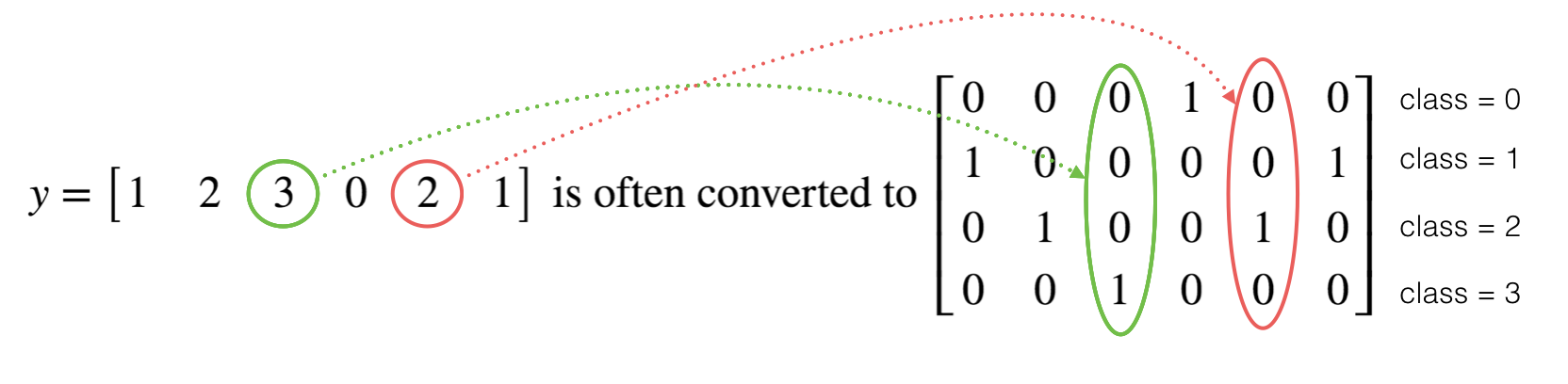
This is called a “one hot” encoding, because in the converted representation exactly one element of each column is “hot” (meaning set to 1).

6. A Few Words about Tensorflow

• Tensorflow is a programming framework used in deep learning
• The two main object classes in tensorflow are Tensors and Operators.
• When you code in tensorflow you have to take the following steps:
  • Create a graph containing Tensors (Variables, Placeholders …) and Operations (tf.matmul, tf.add, …)
  • Create a session
  • Initialize the session
  • Run the session to execute the graph
• You can execute the graph multiple times as you’ve seen in model()
• The backpropagation and optimization is automatically done when running the session on the “optimizer” object.

• Previous
  「译」FAQ：流浪猫对鸟类的影响
• Next
  「Note」Structuring Machine Learning Projects